Stat 7770, Module 03
Richard Waterman
January 2023
Objectives
Objectives
- A first look at the pandas library.
-
The Series container:
-
Selecting components of a Series:
- By position.
- By name.
- By logical filter.
- Statistical summaries.
-
Selecting components of a Series:
Objectives (cont.)
-
The DataFrame container:
- Components of a data frame.
- Creating a data frame from a dict structure.
-
Selecting components of a data frame (rows and columns):
- By position.
- By name.
- By logical filter.
- Using the “.loc” and “.iloc” methods.
- Creating more complex logical filters.
The pandas library
The pandas library
- This is the most popular Python library for data science.
- It provides tools to simplify many parts of the data science workflow.
-
We will look at two special data structures in pandas:
- Series
- DataFrame
- The DataFrame is ideally suited for holding statistical data, because it works in a row/column fashion just like a spreadsheet, and can contain different data types. In particular both numeric and categorical data.
- You can think of a data frame schematically like an Excel or Google Sheets spreadsheet, but you manipulate it programatically, rather than through a graphical user interface (GUI).
The Series container
The Series container
- A series is similar to a Python list structure, but it also has a label for each element, known as the “index”.
- As well as identifying elements by position, you can access them via their labels, or via a logical filter.
- If you don’t specify an index then a default numeric one will be created (starting at 0). Think of it as the row number.
# This will be the standard way of importing the pandas library and aliasing it to "pd"
import pandas as pd

# Create some data in place (later we will import from various sources).
# These are median house prices from various locations around Philadelphia.
house_data = pd.Series([66803, 104923, 114233, 114572, 112471, 99843, 74308, 147176, 199065, 130953],
                      index =['Collindale','Downingtown', 'Falls Town', 'Hatboro', 'Lansdale',
                              'Norwood', 'Sharon Hill', 'Springfield', 'Upper Darby', 'Yardley'])
Review the Series object
- Note that the index is printed along with the house prices.
- The data type, (here int64, means a 64 bit integer) is indicated at the bottom (This is a numeric variable).
- Knowing the data type is useful because the relevant statistical summaries and methods will depend on the data type.
Collindale      66803
Downingtown    104923
Falls Town     114233
Hatboro        114572
Lansdale       112471
Norwood         99843
Sharon Hill     74308
Springfield    147176
Upper Darby    199065
Yardley        130953
dtype: int64
Obtaining just the Series values or just the index
- Use the .values and .index properties/attributes (There are no parentheses after them.)
array([ 66803, 104923, 114233, 114572, 112471,  99843,  74308, 147176,
199065, 130953], dtype=int64)Index(['Collindale', 'Downingtown', 'Falls Town', 'Hatboro', 'Lansdale',
'Norwood', 'Sharon Hill', 'Springfield', 'Upper Darby', 'Yardley'],
dtype='object')Accessing elements in the Series
-
Using pandas there are three ways of accessing the Series elements:
- By position.
- By name.
- By logical filter.
By position:
- You can identify arbitrary elements in the Series by position:
Collindale      66803
Springfield    147176
Hatboro        114572
dtype: int64- If you tried using this notation with a plain list rather than a Series, then …
---------------------------------------------------------------------------

TypeError                                 Traceback (most recent call last)

~\AppData\Local\Temp\ipykernel_11272\522800190.py in <module>
      1 list_a = list(range(10)) # Make a list
----> 2 list_a[[0,7,3]] # This does not work!


TypeError: list indices must be integers or slices, not list
By position as indicated by the slice notation.
Falls Town    114233
Hatboro       114572
Lansdale      112471
dtype: int64
By index label
- Look at the difference in output between using one square bracket and using two square brackets:
104923Downingtown 104923
dtype: int64Getting more than one element by name
- You can obtain arbitrary elements by name:
Downingtown    104923
Lansdale       112471
Upper Darby    199065
Falls Town     114233
dtype: int64
By logical filter
- Rather than using a name or position to extract an element in the Series, you can use a list with logical (True/False) values.
- So long as the list is the same length as the Series, those elements corresponding to a True are selected.
- Think of a logical filter like a sieve, and only those elements lining up with Trues get through.
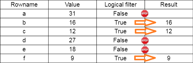
Example
raw_data = pd.Series([31,16,12,27,28,9],
                      index =['a','b', 'c', 'd', 'e','f'])
logic_filter = [False, True, True, False, False, True]

print(raw_data[logic_filter])
b 16
c 12
f 9
dtype: int64Selection by filter for the housing data
# A list containing Trues in positions, 0,3,7,8
logical_list = [True, False, False, True, False, False, False, True, True, False]

house_data[logical_list]
Collindale 66803
Hatboro 114572
Springfield 147176
Upper Darby 199065
dtype: int64Create the logical filter using comparison operators
- Find all the locations where the price is greater than $110,000.
expensive = house_data > 110000 # A logical comparison returning another Series, but this time of logicals.
print(expensive)
Collindale False
Downingtown False
Falls Town True
Hatboro True
Lansdale True
Norwood False
Sharon Hill False
Springfield True
Upper Darby True
Yardley True
dtype: boolSelecting the expensive areas
pandas.core.series.SeriesFalls Town 114233
Hatboro 114572
Lansdale 112471
Springfield 147176
Upper Darby 199065
Yardley 130953
dtype: int64A second example, all on one line
- Find those areas with prices between 90000 and 110000.
- The logical statement can be created within the [] parenthesis as well.
Downingtown    104923
Norwood         99843
dtype: int64
Statistical summaries with pandas
- pandas provides many built in statistical summaries as methods, like mean and median (to be discussed).
116434.7113352.00.25 101113.00
0.50 113352.00
0.75 126857.75
dtype: float64Overwriting elements of the series
- If you can identify parts of a Series, then you can edit/overwrite them using the assignment operator.
Collindale      66803
Downingtown    104923
Falls Town     123456
Hatboro        114572
Lansdale       112471
Norwood         99843
Sharon Hill     74308
Springfield    147176
Upper Darby    199065
Yardley        130953
dtype: int64
Overwriting elements of the series, ctd.
Collindale       66803
Downingtown     104923
Falls Town      123456
Hatboro         114572
Lansdale        999999
Norwood        8888888
Sharon Hill      74308
Springfield     147176
Upper Darby     199065
Yardley         130953
dtype: int64
Overwriting elements of the series, ctd.
house_data[house_data < 100000] = 0 # Overwrite using a logical filter to identify, and a repeated value to populate.
print(house_data)
Collindale 0
Downingtown 104923
Falls Town 123456
Hatboro 114572
Lansdale 999999
Norwood 8888888
Sharon Hill 0
Springfield 147176
Upper Darby 199065
Yardley 130953
dtype: int64Object orientated terminology
- pandas provides a class called Series. It is like an abstract blue print for this data structure.
- Any Series that we create is an object of type Series.
- When we built the specific house_data Series, it is an instance of the Series class.
- The class comes with attributes that are variables defined in the class.
- The class comes with methods that are functions defined in the class.
The DataFrame container
The DataFrame container
- The DataFrame container is a rectangular data structure/container, with rows and columns.
- The columns are usually named, and the rows have an Index.
- Almost all statistical analysis programs use such a structure.
- An important feature of this container is that it can have different data types (numeric, string etc.) in different columns.
- In this way it is able to hold realistic datasets, which are usually of mixed variable types.
The components of a data frame

Creating a DataFrame
- There are a variety of ways to populate a data frame with data, and we will subsequently learn how to read from an external source like a file or database.
- For our first data frame we will input the data ourselves and create the data frame directly.
- The data will come from a dict of lists.
- The keys in the dict will become the column names and the values in the lists will become the entries for each column.
- The data comes from a hospital outpatient clinic, where each row is a patient, the columns are patient attributes and the key variable of interest is Status which indicates whether a patient showed up for their visit.
- Later on we will use a bigger version of this dataset to create a predictive model of whether a patient shows up for their visit.
The raw data
#A dict structure containing the raw data and column names:
raw_data = {'Sex': ['male','female','female','male','female','male','male','female','female','male'],
           'Age': [4,40,23,22,60,50,55,70,58,28],
           'Schedule lag': [41,29,5,18,1,17,29,3,4,2],
           'Schedule minutes':[30,15,30,30,15,10,30,30,15,30],
           'Status': ['No show', 'No show', 'No show', 'No show', 'Show', 'Show', 'No show', 'No show', 'Show', 'No show']}
Populating the data frame
patient_data = pd.DataFrame(data = raw_data) # pd.DataFrame() when passed the raw data will create the new data frame.
print(patient_data)
Sex Age Schedule lag Schedule minutes Status
0 male 4 41 30 No show
1 female 40 29 15 No show
2 female 23 5 30 No show
3 male 22 18 30 No show
4 female 60 1 15 Show
5 male 50 17 10 Show
6 male 55 29 30 No show
7 female 70 3 30 No show
8 female 58 4 15 Show
9 male 28 2 30 No showFinding the size of the data frame and the types of variables included
(10, 5)Sex object
Age int64
Schedule lag int64
Schedule minutes int64
Status object
dtype: object- When the data type is listed as “object” this means it is being treated as a string type, so statistically, the column will be viewed as a categorical variable.
Review the column names
- We already know the column names of this data frame, but when you read in from an external source that is not always the case.
- The column names can be identified through the .columns attribute.
- Notice the names are in what is called an “Index” object. An index contains information about the rows or columns, for example, their names.
## Get just the names of the columns in the data frame with the .columns attribute.
print( patient_data.columns)
Index(['Sex', 'Age', 'Schedule lag', 'Schedule minutes', 'Status'], dtype='object')Selecting pieces of the data frame
- We will be interested in subsetting by rows and subsetting by column, or possibly both.
- The most basic operation is to get at a specific column, and here is a direct way to do it:
# Get the Age column by name as we would if the data structure were a dict.
print(patient_data['Age'])
0 4
1 40
2 23
3 22
4 60
5 50
6 55
7 70
8 58
9 28
Name: Age, dtype: int64Getting at the column, using the name as an attribute
0     4
1    40
2    23
3    22
4    60
5    50
6    55
7    70
8    58
9    28
Name: Age, dtype: int64Adding an index for the rows
- The data frame was created with default row names, the numbers 0 through 9.
RangeIndex(start=0, stop=10, step=1)Creating the new index
- If we had patient identifiers we could use these instead for the row index.
- Below, we create some patient identifiers and add them to the data frame as an index.
- We also give a name “Patient ID” to the new index.
patient_ids = ['P456', 'P126','P563', 'P884','P102', 'P067','P120', 'P943','P496', 'P805'] # Patient identifiers.
patient_data.index = patient_ids # Assign a new index.
patient_data.index.name = 'Patient ID' # Give the new index a name.
print(patient_data) # Check out the data frame.
Sex Age Schedule lag Schedule minutes Status
Patient ID
P456 male 4 41 30 No show
P126 female 40 29 15 No show
P563 female 23 5 30 No show
P884 male 22 18 30 No show
P102 female 60 1 15 Show
P067 male 50 17 10 Show
P120 male 55 29 30 No show
P943 female 70 3 30 No show
P496 female 58 4 15 Show
P805 male 28 2 30 No showSelecting rows and columns
- There are a variety of ways of selecting rows and columns from the data frame.
- Some are similar to techniques we have seen earlier, but the .loc and .iloc methods are new.
               Sex  Age  Schedule lag  Schedule minutes   Status
Patient ID
P884          male   22            18                30  No show
P102        female   60             1                15     Show
P067          male   50            17                10     Show
Selecting rows and columns
               Sex  Age  Schedule lag  Schedule minutes   Status
Patient ID
P805          male   28             2                30  No show
P496        female   58             4                15     Show
P943 female 70 3 30 No show Sex Status
Patient ID
P456 male No show
P126 female No show
P563 female No show
P884 male No show
P102 female Show
P067 male Show
P120 male No show
P943 female No show
P496 female Show
P805 male No showUsing the locate methods
- The first, “.loc” allows to identify by name, and the second “.iloc” by integer location.
             Sex  Age  Schedule lag  Schedule minutes   Status
Patient ID
P120        male   55            29                30  No show
P805 male 28 2 30 No show Sex Status
Patient ID
P120 male No show
P805 male No showIdentifying by position
- The two statements below look very similar, but one has [] and the other [[]].
- The first returns a Series and the other one, a single column DataFrame.
Sex                  female
Age                      40
Schedule lag             29
Schedule minutes         15
Status              No show
Name: P126, dtype: object Sex Age Schedule lag Schedule minutes Status
Patient ID
P126 female 40 29 15 No showSelecting the first and last rows of the data frame
Sex Age Schedule lag Schedule minutes Status
Patient ID
P456 male 4 41 30 No show
P805 male 28 2 30 No showSelecting multiple rows and columns
Schedule lag Schedule minutes
Patient ID
P126 29 15
P884 18 30
P067 17 10 Schedule minutes Status
Patient ID
P456 30 No show
P126 15 No showUsing logical filters
- Just like with Series, it can be important to select rows from a data frame with specific attributes.
- For example, just select the males, or just select the females.
- This can be done in the same was we did for the Series data structure.
patient_data.Sex == "female" # A series where the trues are for females and the falses for males.
print(patient_data.Sex == "female")Patient ID
P456 False
P126 True
P563 True
P884 False
P102 True
P067 False
P120 False
P943 True
P496 True
P805 False
Name: Sex, dtype: boolSelecting just the female rows from the data frame
               Sex  Age  Schedule lag  Schedule minutes   Status
Patient ID
P126        female   40            29                15  No show
P563 female 23 5 30 No show
P102 female 60 1 15 Show
P943 female 70 3 30 No show
P496 female 58 4 15 Show# A compound selection of females who showed up. The "&" here performs the logical "and".
# It works elementwise on the two boolean Series.
print(patient_data[(patient_data.Sex == "female") & (patient_data.Status == "Show")]) Sex Age Schedule lag Schedule minutes Status
Patient ID
P102 female 60 1 15 Show
P496 female 58 4 15 ShowLogical selection together with column extraction
- We could combine logical selection with column selection, to get at specific columns for which conditions hold true on other columns.
# Get the schedule lag for females who showed up.
print(patient_data[(patient_data.Sex == "female") & (patient_data.Status == "Show")].iloc[:, [2]])
Schedule lag
Patient ID
P102 1
P496 4Editing/overwriting parts of a data frame
- As with Series, if you can select a part of a data frame, you can edit through assignment.
print(patient_data.iloc[2,0]) # Sex of the third patient.
patient_data.iloc[2,0] = 'male' # Overwrite from female to male.
print(patient_data.iloc[2,0])
female
maleEditing a row slice
               Sex  Age  Schedule lag  Schedule minutes   Status
Patient ID
P456          male    4            41                30  No show
P126        female   40            29                15  No show
P563          male   19             5                30  No show
P884          male   19            18                30  No show
P102        female   60             1                15     Show
P067          male   50            17                10     Show
P120          male   55            29                30  No show
P943        female   70             3                30  No show
P496        female   58             4                15     Show
P805          male   28             2                30  No show
Editing rows and columns simultaneously
- Note the nested lists being used for each row.
               Sex  Age  Schedule lag  Schedule minutes   Status
Patient ID
P456            NA   99            41                30  No show
P126        female   40            29                15  No show
P563          male   19             5                30  No show
P884            NA   99            18                30  No show
P102        female   60             1                15     Show
P067          male   50            17                10     Show
P120          male   55            29                30  No show
P943        female   70             3                30  No show
P496        female   58             4                15     Show
P805          male   28             2                30  No show
Class summary
Summary
- A first look at the pandas library.
-
The Series container:
- Selecting components of a Series.
- Statistical summaries.
-
The DataFrame container:
- Components of a data frame.
- Creating a data frame from a dict structure.
- Selecting components of a data frame (rows and columns).
- Creating more complex logical filters.
Next time
Next time
-
Importing data to Python:
- Data file types.
- CSV.
- HTML.
- JSON.
-
Data locations:
- A local file.
- A remote (web) resource.
- A database.
- Joining datasets.
- Dates and times