SMMD, Term 1, 2003, Class 13

What you need to have learned from class 12

Adding categorical variables to a regression.

Two basic models:

No interaction: the impact of X1 on Y does not depend on the level of X2.

Interaction: the impact of X1 on Y depends on the level of X2.

Practical consequences:

If NO interaction, then you can investigate the impact of each X by itself.

If there is interaction (consider practical importance as well as statistical significance) then you must consider both X1 and X2 together.

New material for today

Regression for a categorical response.

A loose end - log transforms

Note: all percent change interpretations for log transforms are valid only if the percent change considered is small. The smaller it is the better the approximation.

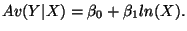
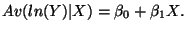
Four cases:

$Av(Y\vert X) = \beta_0 + \beta_1 X.$

$Av(Y\vert X) = \beta_0 + \beta_1 ln(X).$

$Av(ln(Y)\vert X) = \beta_0 + \beta_1 X.$

$Av(ln(Y)\vert X) = \beta_0 + \beta_1 ln(X).$

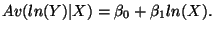
Four respective interpretations for $\beta_1$:

For a 1 unit change in X, the average of Y changes by $\beta_1$.

For a 1 percent change in X, the average of Y changes by $\beta_1/100$.

For a 1 unit change in X, the average of Y changes by 100 $\beta_1$ percent.

For a 1 percent change in X, the average of Y changes by $\beta_1$ percent - the economist's elasticity definition.

A link to the math

Plug in numbers if in doubt: take $\beta_0 = 5$ and $\beta_1 = 0.5$.

$Av(ln(Y)\vert X) = 5 + 0.5 ln(X).$

Calculate Av(ln(Y)) at X = 100: $ln(Y) = 5 + 0.5 \times ln(100) = 7.3026$, so Y = 1484.13

Increase X by 1% (X = 101) and recalculate: 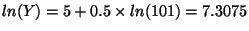$ln(Y) = 5 + 0.5 \times ln(101) = 7.3075$, so Y = 1491.53

Y has gone from 1484.13 to 1491.53, or in percent terms: (1491.53 - 1484.13)/1484.13 = 0.00498 = 0.498%, which is approximately 0.5%.

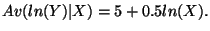
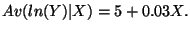
Plug in numbers if in doubt: take $\beta_0 = 5$ and $\beta_1 = 0.03$.

$Av(ln(Y)\vert X) = 5 + 0.03 X.$

Calculate Av(ln(Y)) at X = 50: 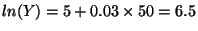$ln(Y) = 5 + 0.03 \times 50 = 6.5$, so Y = 665.14

Increase X by 1 (X = 51) and recalculate: 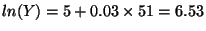$ln(Y) = 5 + 0.03 \times 51 = 6.53$, so Y = 685.40

Y has gone from 665.14 to 685.40, or in percent terms: (685.40 - 665.14)/665.14 = 0.0305 = 3.05%, which is approximately 3%.

Simple Logistic Regression. Chapter 11

Objective: model a categorical (2-group) response.

Example: how do gender and income impact the probability of the purchase of a product.

Estimate probabilities that someone responds to a direct mail shot.

Classify customers into 2 segments, those with a high chance of purchasing, and those with a low chance.

Problem: linear regression does not respect the range of the response data (it's categorical).

Solution: model the probability that Y = 1, ie P(Y = 1 | X), in a special way.

Transform P(Y = 1) with the ``logit'' transform.

Now fit a straight line regression to the logit of the probabilities (this respects the range of the data).

On the original scale (probabilities) the transform looks like this:

The logit is defined as logit(p) = ln(p/(1-p)). Example logit(.25) = ln(.25/(1 - .25)) = ln (1/3) = -1.099.

The three worlds of logistic regression.

The probabilities: this is where most people live.

The odds: this is where the gamblers live.

The logit: this is where the model lives.

Must feel comfortable moving between the three worlds.

Rules for moving between the worlds. Call P(Y = 1|X), p for simplicity.

logit(p) = ln(p/(1-p))

p = exp(logit(p))/(1 + exp(logit(p))) *** Key to get back to the real world.

odds(p) = p/(1-p)

odds(p) = exp(logit(p)) *** Key for interpretation.

Interpreting the output.

P-values are under the Prob>ChiSq column.

Main equation logit(p) = B0 + B1 X.

B1: for every one unit change in X, the ODDS that Y = 1 changes by a multiplicative factor of exp(B1).

B1 = 0. No relationship between X and p.

B1 > 0. As X goes up p goes up.

B1 < 0. As X goes up p goes down.

At X = -B1/B0 there is a 50% chance that Y = 1.

Key calculation - based on the logistic regression output calculate a probability. Example: Challenger output on pp.281-282.

logit(p) = 15.05 - 0.23 Temp.

Find the probability that Y = 1 (at least one failure) at a temperature of 31.

logit(p) = 15.05 - 0.23 * 31

logit(p) = 7.96.

p = exp(logit(p))/(1 + exp(logit(p)))

p = exp(7.96)/(1 + exp(7.96)) = 0.99965

The model indicates that there is a 99.965 percent chance of at least one failure.