HiGrad: Hierarchical Incremental GRAdient Descent
 |
HiGrad is a first-order algorithm for finding the minimizer of a function in online learning just like SGD and, in addition, this new method attaches a confidence interval to assess the uncertainty of its predictions. |
Paper
Uncertainty Quantification for Online Learning and Stochastic Approximation via Hierarchical Incremental Gradient Descent
Stochastic gradient descent (SGD) is an immensely popular approach for online learning in settings where data arrives in a stream or data sizes are very large. However, despite an ever-increasing volume of work on SGD, much less is known about the statistical inferential properties of SGD-based predictions. Taking a fully inferential viewpoint, this paper introduces a novel procedure termed HiGrad to conduct statistical inference for online learning, without incurring additional computational cost compared with SGD. The HiGrad procedure begins by performing SGD updates for a while and then splits the single thread into several threads, and this procedure hierarchically operates in this fashion along each thread. With predictions provided by multiple threads in place, a \(t\)-based confidence interval is constructed by decorrelating predictions using covariance structures given by the Ruppert–Polyak averaging scheme. Under certain regularity conditions, the HiGrad confidence interval is shown to attain asymptotically exact coverage probability. Finally, the performance of HiGrad is evaluated through extensive simulation studies and a real data example. An R package higrad has been developed to implement the method.
Code & Data
An R package implementing HiGrad is available at Yuancheng's github.
Code and data used to generate figures in the paper.
Outline
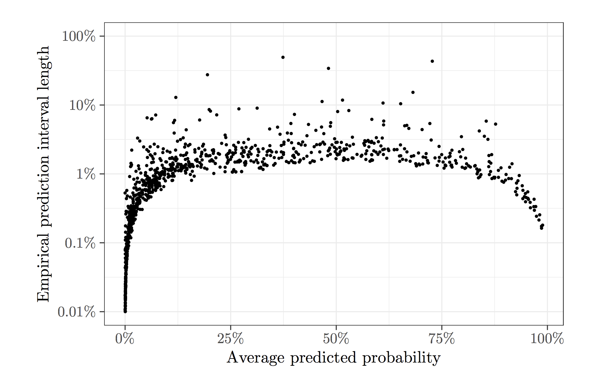
Stochastic gradient descent (SGD) always yields noisy predictions, and sometimes the uncertainty of its predictions can be significant. To illustrate this, we apply SGD to the Adult dataset hosted on the UCI Machine Learning Repository as an example, which contains demographic information of a sample from the 1994 US Census Database. We use logistic regression to predict whether a person's annual income exceeds $50,000. To fit the logistic regression model, we run SGD for 25 epochs (approximately 750,000 steps of SGD updates) and use the estimated model to predict for a random test set of 1,000 units. The procedure is repeated for a total of 500 times, and the plot below shows the length of the 90%-coverage empirical prediction interval against the average predicted probability for each sample unit. There are a fair proportion of the test sample units with a large variability near 50%. This is the regime where variability must be addressed since the decision based on predictions can be easily reversed.
A confidence interval is used to evaluate the uncertainty of random predictions. In settings where data arrive in an online fashion, HiGrad is designed to attach a confidence interval to its prediction. To briefly introduce this online setting, let \(f(\theta)\) be a smooth convex function defined on a Euclidean space and denote by \(\theta^\ast\) its unique minimizer. Suppose an iid sample \(Z_1, Z_2, \ldots, Z_N\) are observed sequentially. For each unit \(Z_i\), we have access to an unbiased noisy gradient \(g(\theta, Z_i)\) that obeys \(\mathbb{E} g(\theta, Z_i) = \nabla f(\theta)\).
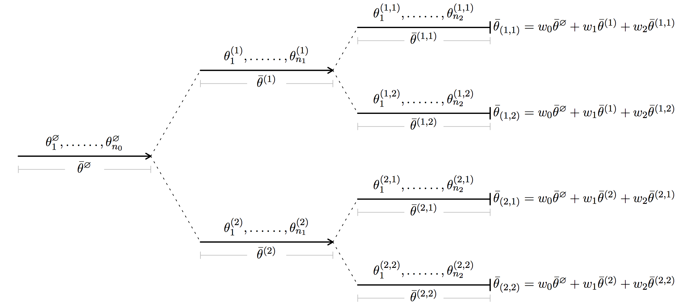
In short, HiGrad is performing SGD iterations on a tree. This point is best illustrated by the diagram above. Along the first segment, HiGrad performs iterations
\[ \theta_j^{\emptyset} = \theta_{j-1}^{\emptyset} - \gamma_j g(\theta_{j-1}^{\emptyset}, Z_j^{\emptyset}) \]
for \(j = 1, \ldots, n_0\), initialized at \(\theta_0^{\emptyset} = \theta_0\). Above, \(\gamma_j\) is the step size or, put differently, the learning rate. At the end of the segment, the iteration is split into two segments. Each of the two segments continues to perform the SGD iterations starting from \(\theta_0^{\emptyset}\), but feed on disjoint data streams. As shown in the diagram, each of the two segments is further split into two segments, resulting in \(T = 4\) paths between the root and a leaf. A path here is referred to as a thread. The total length of all the segments is \(N\), the number of all sample units. Thus, we see
HiGrad is online in nature, with the same computational cost as SGD.
To make use of the HiGrad iterates, define the averaged iterates
\[ \overline \theta^{b} = \frac1{n_k} \sum_{j=1}^{n_k} \theta^{b}_j. \]
for each segment \(b\) and
\[ \overline \theta_{t} = \sum_{k=0}^K w_k \overline \theta^{(b_1, \ldots, b_k)}. \]
for each thread \(t\), where \(w\) is a vector of weights. Let \(\mu_x\) be the (smooth) prediction function. With a bit abuse of notation, \(\mu_x \in \mathbb{R}^T\) is also used to denote a \(T\)-dimensional vector consisting of all \(\mu_x^{t} := \mu_x(\overline\theta_{t})\), and write \(\mu_x^\ast = \mu_x(\theta^\ast)\) for short. Since different threads share some segments at the beginning, entries of \(\mu_x\) are correlated with each other. To recognize the correlation structure of the \(T\) threads, note that for two different threads \(t = (b_1, \ldots, b_K)\) and \(t’ = (b_1’, \ldots, b_K’)\) with \(1 \le b_k, b_k’ \le B_k\) for \(k = 1, \ldots, K\), the number of data points shared by \(t\) and \(t'\) vary from \(n_0\) to \(n_0 + n_1 + \cdots + n_{K-1}\). Intuitively, the more they share, the larger the correlation is. Loosely speaking, as the length of the data stream \(N \rightarrow \infty\), under certain conditions (local strong convexity at \(\theta^\ast\), Lipschitz gradient, etc) the vector \(\mu_x\) is asymptotically normally distributed with mean \(\mu_x^\ast {\bf 1}: = (\mu_x^\ast, \mu_x^\ast, \ldots, \mu_x^\ast)^\top\) and covariance proportional to \(\Sigma \in \mathbb R^{T \times T}\). The proof of this result is based on the celebrated Ruppert–Polyak normality result for averaged SGD iterates (developed by David Ruppert, Boris Polyak, and Anatoli Juditsky in the late 80s and early 90s). The covariance \(\Sigma\) is given as
\[ \Sigma_{t, t’} = \sum_{k=0}^p \frac{w_k^2 N}{n_k} \]
for any two threads \(t, t'\) that agree exactly on the first \(p\) segments. Making use of this distributional property, we propose an estimator of \(\mu_x^\ast\) that takes the form
\[ \overline \mu_x := \frac1T \sum_{t \in \mathcal{T}} \mu_x^{t} \]
and a \(t\)-based confidence interval
\[ \left[ \overline\mu_x - t_{T - 1, 1-\frac{\alpha}{2}}\mathrm{se}_x, \quad \overline\mu_x + t_{T - 1, 1-\frac{\alpha}{2}}\mathrm{se}_x \right] \]
at nominal level \(1 - \alpha\). The standard error \(\mathrm{se}_x\) is given as
\[ \mathrm{se}_x = \sqrt{\frac{{\bf 1}^\top \Sigma {\bf 1} \, (\mu_x^\top - \overline\mu_x \, {\bf 1}^\top) \Sigma^{-1} (\mu_x - \overline\mu_x \, {\bf 1})}{T^2(T - 1)}}. \]
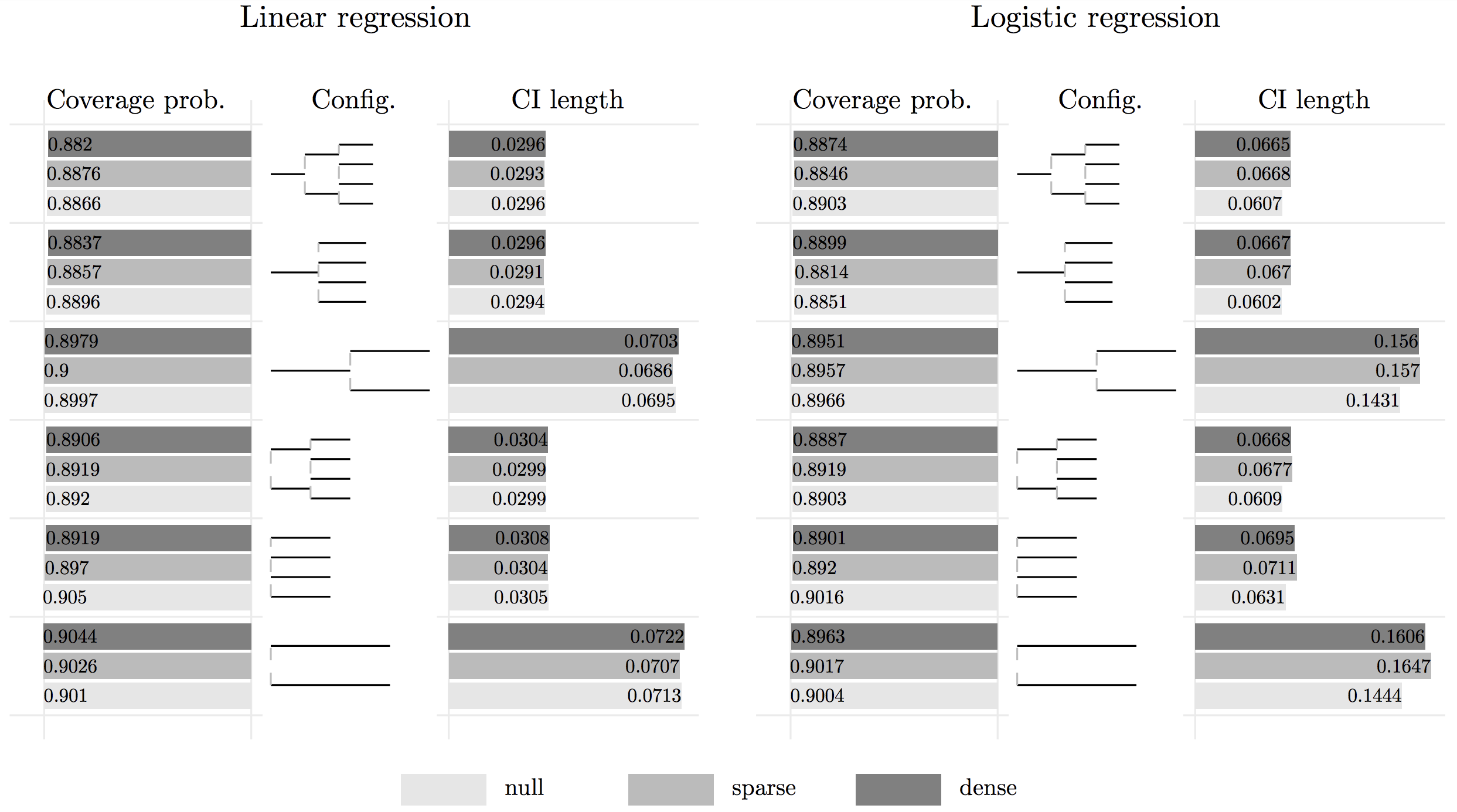
Below presents a bar plot of a simulation study of applying HiGrad with different configurations. For both linear regression and logistic regression, HiGrad is shown to achieve a coverage probability that is very close to the nominal level 90%. Thus, we conclude
In addition to an estimator, HiGrad gives a confidence interval for \(\mu_x^\ast\).
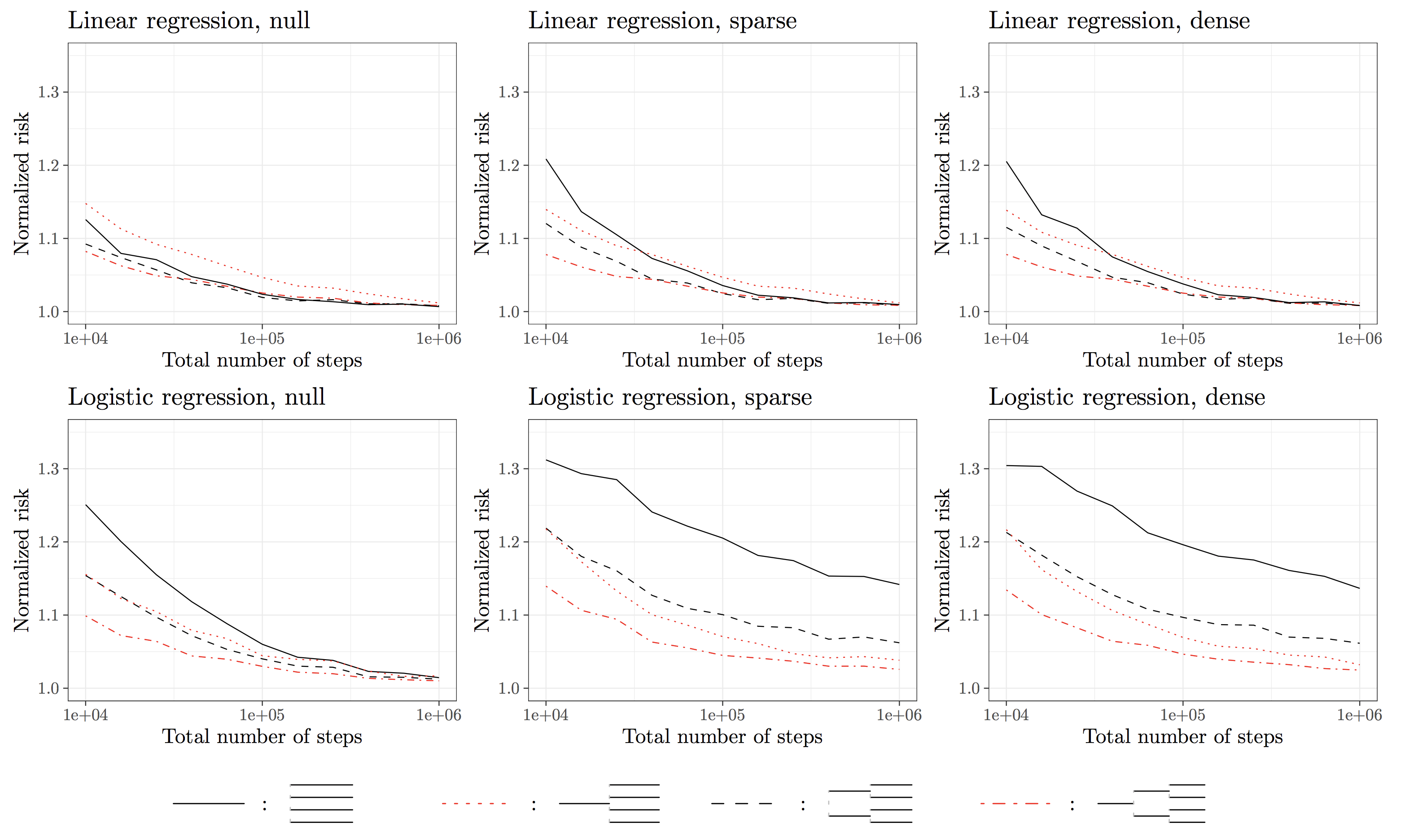
So far, one question remains unaddressed. What is the accuracy of the HiGrad predictions compared with that of SGD? To get a sense of this pressing question, we conduct a simulation study summarized in the following plot. The HiGrad risk is normalized by the SGD risk, and we vary the number iterations from \(10^4\) to \(10^6\). From the plot, the dash-dotted red line, which corresponds to the HiGrad configuration with two splits, quickly tends to 1 as the number of iterations gets large. This implies that only a small fraction of efficiency is lost in using HiGrad instead of SGD. To summarize, we get
The HiGrad estimation is almost as accurate as that of SGD under certain conditions.
Talks
Joint Statistical Meetings (7/2018)
IMS Asia Pacific Rim Meeting in Singapore (6/2018)
ICSA Applied Statistics Symposium (6/2018)
Workshop Series on Statistical Scalability, Isaac Newton Institute (4/2018)
52nd Annual Conference on Information Sciences and Systems (CISS) (3/2018)
Princeton Wilks Memorial Seminar in Statistics (Yuancheng, 3/2018)
Penn Research in Machine Learning Seminar (1/2018)
Fudan Data Science Conference (12/2017)
Young Mathematician Forum, Peking University (12/2017)
Tsinghua IIIS Seminar (12/2017)
Fudan Economics Seminar (12/2017)
Berkeley Neyman Statistics Seminar (12/2017)
Stanford Statistics Seminar (12/2017)
New Jersey Institute of Technology Statistics Seminar (11/2017)
Binghamton University Statistics Seminar (11/2017)
Penn ESE Colloquium (10/2017)
Rutgers University Statistics Seminar (10/2017)